Tutorial: Formatting parameter maps in GIS

This section describes how to prepare parameter maps for input to Vflo™. Step-by-step tutorial instructions walk the user through developing the following parameter maps in GIS:

1. Flow direction map derived from a high resolution DEM

2. Channel base width map

3. Channel side slope map

4. Slope map

5. Roughness map

6. Infiltration parameter maps

a. Hydraulic conductivity

b. Wetting front suction

c. Effective porosity

7. Impervious map

These tutorial instructions guide users through the GIS development steps needed to prepare model parameter maps in a common projection and for a common domain. For tutorial purposes, the ASCII parameter maps exported in this section may subsequently be used for assembly of a sample Vflo™ model. Keep in mind, however, that if AutoBOP is used, the amount of GIS pre-processing required is greatly reduced. AutoBOP automates many of the manual development processes that were previously required, and that are described in detail below. With AutoBOP, a flow direction map is internally processed from DEM data. The Vflo™ domain is custom-fit to user specifications, and parameter maps are automatically re-projected to a target Vflo™ coordinate system.

Developing parameter maps in GIS is necessary because parameter data such as soil maps and landuse maps usually cannot be input directly to Vflo™. Vflo™ uses GIS maps to set parameter values in thousands of cells at once. This makes the modeling of large areas at high resolution possible. However, landuse, soils, and digital elevation models are usually developed without regard for the needs of a hydrologic model. Vflo™ expects data and values in specific formats for use in its numerical solution. Because data is formatted differently for a variety of purposes and applications, it may need to be modified for use in Vflo™.

Selecting appropriate GIS software

The following step-by-step tutorial instructions utilize ArcGIS 9.2 with Spatial Analyst. GIS parameter maps for Vflo™ may also be developed using ArcView 3.2 with Spatial Analyst, ArcGISx with Spatial Analyst, or other GIS software such as WMS. AutoBOP may be used to process the flow direction map and re-project files.

Using alternative parameter map development methods

The directions included are only one example of how to prepare data for Vflo™; each step shown could be accomplished through a variety of methods. Because stream channels and slopes derived from DEMs may contain artifacts that result from regular sampling of an irregular elevation surface at coarse resolution, suggested methods are offered to help enhance data quality. However, the user should apply methods that are appropriate for their specific watersheds.

The instructions also assume use of a DEM for deriving flow direction, and availability of landuse and soil maps for defining hydraulic roughness and infiltration values. There are alternatives to these methods, however. A flow direction map may be drawn manually, rather than derived from a digital elevation model (DEM). In addition, if gridded data is not available for defining infiltration, roughness, and other parameter values, then constant values may be assigned for a watershed or sub-areas that are representative of the local conditions.

Parameter map formatting requirements

When parameter maps are loaded using AutoBOP, ASCII parameter files may be established in different coordinate systems. AutoBOP has the capability to reproject each file to a designated target coordinate system. If parameter maps are loaded outside of AutoBOP, however, the following formatting requirements apply:

1. 
   Horizontal units must be in meters, regardless of whether metric or US customary units are being used.
2. Vertical units must either be all in metric units, or all in US customary units.
3. All Vflo™ parameter maps must be in ESRI ASCII GRID file format.
4. The same domain extent, or number of rows and columns, and the same lower left x,y coordinates as the flow direction map must be used for all ESRI ASCII GRID files. This means that all datasets will need to be:

a. Clipped to the same domain

b. Sampled to the same grid cell size, and

c. Projected in the same projection

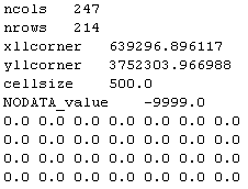
Domain and resolution information can be found in the header of any ESRI ASCII GRID files, as shown in the above right image. ASCII file headers describe the number of columns ("ncols"), the number of rows ("nrows"), the lower left x-coordinate ("xllcorner"), the lower left y-coordinate ("yllcorner"), and the resolution ("cellsize").

Sample data

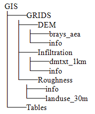
Locate and make a copy of the Brays Bayou, TX sample data that is provided online at http://apps.vieuxinc.com/sampleData/Example_GIS.zip. The sample data files will be named as shown at right. The sample data is to be used as a learning tool as the user follows the tutorial instructions. The sample parameter data are useful for demonstrating how to prepare parameter maps for use in Vflo™; when Vflo™ parameters are set up for other watersheds, however, parameter information that is representative of the particular watershed being modeled must be used.

Setting up ArcGIS for developing parameter maps

These instructions describe the basic steps needed to set up ArcGIS for preparing Vflo™ parameter maps. Steps include: opening a new empty map in ArcMap, selecting the Spatial Analyst extension and viewing the Spatial Analyst toolbar, and setting the data frame projection and working directory.

Tutorial instructions

1. Start ArcMap.

Within the ArcMap window, select “Start using ArcMap with A new empty map.” Click OK.

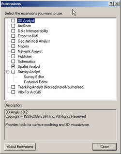
Then, find the Tools menu in the menu bar at the top of the screen. Under Tools | Extensions, select Spatial Analyst.

2. 

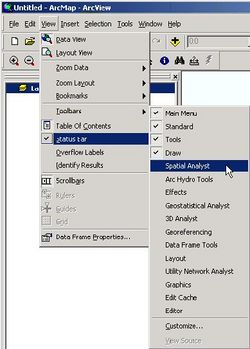
Under View | Toolbars, select Spatial Analyst.

The Spatial Analyst toolbar will appear.

3. 

Set the data frame projection.

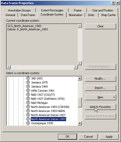
Right click on the data frame Layers. Select Properties. The Data Frame Properties window will appear. Click on theCoordinate System tab, as shown at right.

Navigate to a shapefile or grid that contains the same projection information that you will use for all subsequent datasets and click Add. Or, define a coordinate system by clicking on the New button.

The projection name and information should now appear in the field titled Current coordinate system. Click Add to Favoritesand then OK.

4. 

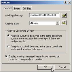
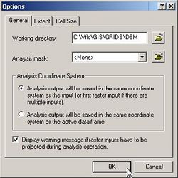
Set the working directory under Spatial Analyst.

Under Spatial Analyst | Options | General, click on the Open  button next to the Working Directory field and navigate to the folder that will serve as a directory. Files generated in ArcGIS will be saved to this folder. Click OK.

Flow direction

Before using this section, see Parameter map formatting requirements for general ASCII formatting instructions.

Producing a flow direction map is the first step in generating a Vflo™ model. This section includes tutorial instructions for using GIS software to produce a flow direction map for input to Vflo™. Rather than using GIS software to manually develop a flow direction map outside of Vflo™, a high resolution DEM may be input to AutoBOP to automatically develop flow direction parameters directly within Vflo™. In addition, if a DEM is not available, a flow direction map may be drawn manually in Vflo™.

A high resolution DEM and GIS software are required. The instructions utilize ArcGIS 9.2 with Spatial Analyst, but GIS parameter maps for Vflo may also be developed using ArcView 3.2 with Spatial Analyst, ArcGISx with Spatial Analyst, or other GIS software such as WMS. The directions included are only one example of how to prepare a flow direction map for Vflo™. Each step shown could be accomplished through a variety of methods, and the user should apply methods that are appropriate for their specific watershed(s).

The digital elevation model (DEM) is the source of Vflo™ flow direction and slope information. When a sufficiently high resolution DEM is used, the DEM may also be the source of Vflo™ channel location information. Because DEM resolution is often coarser than stream channel data, however, a stream channel map may be used in conjunction with a DEM, as in these tutorial instructions, to force appropriate flow directions near channels. Examples of areas that may not be well defined by a DEM include: braided streams, alluvial fans, flat areas, cutoff-meanders, and multiple channels that may carry flow under certain conditions.

Tutorial instructions

1. 

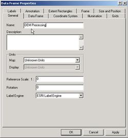
Change the name of the data frame from Layers to DEM Processing.

Right click on Layers, then select Properties | General. Enter "DEM Processing" in the Name field and click OK.

2. 

Assign the projection of the DEM.

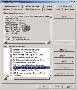
Right click on the data frame DEM Processing, select Properties | Coordinate System | Predefined | Projected Coordinate System.

Under Projected Coordinate System | Continental | North America, select the projection USA Contiguous Albers Equal Area Conic USGS version.

3. 

Set the working directory under Spatial Analyst.

Under Spatial Analyst | Options | General, click on the folder icon next to the Working Directory field and navigate to this path:\GIS\GRIDS\DEM. Click OK.

4. 

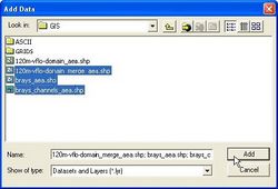
To load shapefiles, click the Add Data  button located on the Standard Toolbar.

Add these shapefiles located in the GIS folder : brays_aea, brays_channels_aea, and 120m-vflo-domain_aea.

5. To load the DEM, click the Add Data  button again.

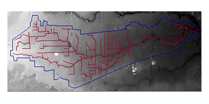
Navigate to the DEM file: \GIS\GRIDS\DEM. Select brays_aea and click Add. Adjust layers as needed for desired display. The resulting display may resemble the image below.

6. 

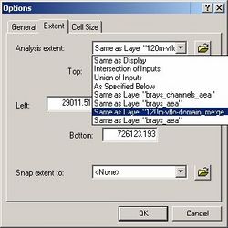
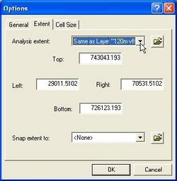
Set the extent to correspond with the Vflo™ domain.

Select Spatial Analyst | Options | Extent. For Analysis extent, choose: Same as Layer “120m-vflo-domain_aea” from the drop down menu.

7. 

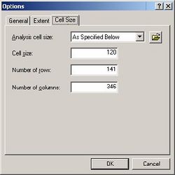
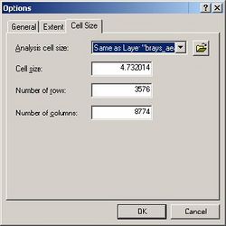
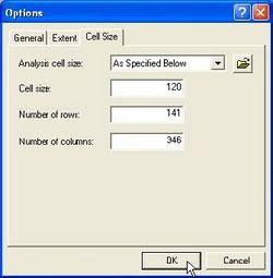
Set the Analysis cell size.

Remaining within Spatial Analyst | Options, click on the Cell Size tab. Select As Specified Below for Analysis cell size. Enter “120” in the Cell Size field.

Click the General tab and make sure that the Working Directory is still set to \GIS\GRIDS\DEM.

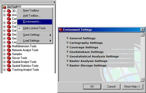
8. Set the Output Vflo™ domain and resolution under the ArcToolbox environment settings.

Open the Arc Toolbox by clicking on the ArcToolbox  button, located in the Standard toolbar. If the Standard toolbar is not shown, select View|Toolbars|Standard.

Within the Arc Toolbox, right click on ArcToolbox, then select Environments│General Settings.

.

 

9. 

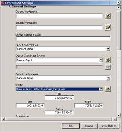
Scroll down to the Extent field.

Select Same as layer 120m-vflo-domain_aea from the drop down menu.

10. 

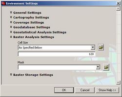
Scroll up and click General Settings again to close the General Settings menu.

Now, click Raster Analysis Settings. Select As Specified Below from the Cell Size drop down menu and enter “120” in the field below the drop down menu.

11. Save the project in the directory desired by selecting File│Save.

12. 

Within the Arc Toolbox, resample the 5m DEM to 120m.

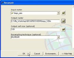
Select ArcToolbox | Data Management Tools | Raster | Resample. In the Resample window, select brays_aea for Input Raster. Browse to GIS\GRIDS\DEM for Output Raster.

Add “brays_120m” to the end of the Output Raster entry so that it reads: “...GIS\GRIDS\DEM\brays_120m”. This effectively names the resampled DEM brays_120m. Enter “120” in the Output Cell Size field and choose BILINEAR for the Resampling Technique.

13. 

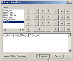
The resampled 120m DEM does not match the desired Vflo™ domain.

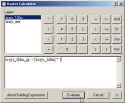
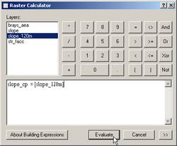
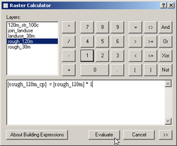
Select Spatial Analyst│Raster Calculator. Within the Raster Calculator window, enter the following expression:

brays_120m_cp = [brays_120m] * 1

To enter the expression, click in the field provided and type “brays_120m_cp.” Then, click the “=” sign, double click onbrays_120m within the Layers field, click the Multiply  button, and click the 1  button. Each term of the expression will appear in the lower field of the Raster Calculator window.

Click Evaluate. Some time may be needed for processing.

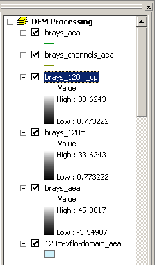
The re-evaluated DEM will appear as a new layer called brays_120m_cp within the Table of Contents, as shown at right.

14. 

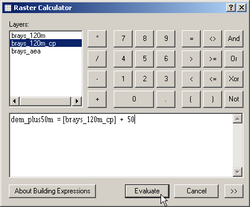
Use the Raster Calculator to add 50m to the resampled DEM.

Select Spatial Analyst│Raster Calculator again. Enter “dem_plus50m”, click the = button, double click on brays_120m_cp, then click the Add button, the 5 button, and the 0 button.

Finally, click Evaluate. This effectively raises all elevations of the DEM by 50m. The output DEM will appear as a new layer within the Table of Contents named dem_plus50m.

15. 

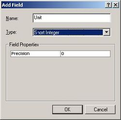
Shapefiles used to enforce streams must have a unit field with a value of ‘1’.

Prepare the stream shapefile brays_channels_aea by adding a unit field. Right click on the brays_channels_aea layer and select Open attribute table. Click the Options button and select Add Field. Type “Unit” in the Name field and select Short Integer for the Type.

16. 

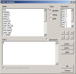
Use the Field Calculator to fill the Unit fields.

Open the attribute table as before. Right click on the Unit column heading and select Field Calculator. Within the Field Calculator window, select Unit for Fields, Number for Type, and enter “1” in the Unit = field. Click OK.

17. 

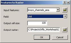
Convert the stream shapefile to a grid.

Select Spatial Analyst | Convert | Feature to Raster. Select brays_channels_aea as Input feature and Unit as Field. Enter “120” (or your desired length) as Output cell size, and navigate to this path for Output Raster: \GIS\GRIDS\DEM\str_unit. The new grid will appear as a layer in the Table of Contents named str_unit.

18. Repeat Steps 12-14 for the shapefile brays_aea, as follows.

Open the attribute table of the brays_aea shapefile, click Options, and select Add Field. Enter Unit for Name and Short Integer for Type, then click OK.

Next, open the attribute table and use the field calculator to fill the Unit field added to the stream shapefile. Right click on the Unit column heading and select Field Calculator. Within the Field Calculator window, select Unit for Fields, Number for Type, and enter “1” in the Unit = field. Click OK.

Finally, convert the basin shapefile to a grid using Spatial Analyst | Convert | Features to Raster. Select brays_aea as Input feature and Unit as Field. Enter “120” (or your desired length) as Output cell size, and navigate to this path for Output Raster: \GIS\GRIDS\DEM\basin_unit. The new grid will appear as a layer in the Table of Contents named basin_unit.

 

19. 

Create a new grid that will contain DEM values only where the stream grid cells exist.

Use the Raster Calculator to multiply brays_120m_cp by str_unit. The resulting DEM may be named str_dem.

20. 

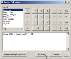
Create a basin wall 100m high around the perimeter of the basin using the unit basin grid.

Keep in mind that, in general, the height of the wall must be larger than the maximum value in the raised DEM.

Use the Raster Calculator to multiply the unit basin grid by 100, naming the resulting layer basin_100m. This grid will be used later when all grids are merged together.

21. 

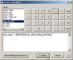
Merge the 100m basin grid (basin_100m) with the raised DEM grid (dem_plus50m).

Enter this expression in the Raster Calculator:

dem_mrg1 = MERGE([basin_100m],[dem_plus50m])

First type in “dem_mrg1” and click the = button. Then type “MERGE”, followed by an open parentheses mark. Double click onbasin_100m, enter a comma, enter a space, then double click on dem_plus50m. Enter a final close parentheses mark and click Evaluate.

22. 

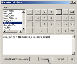
Merge the stream DEM (str_dem) with the walled and raised DEM (dem_mrg1).

This effectively forces the appropriate drainage direction along the stream cells.

Use the Raster Calculator to evaluate the following equation:

dem_merge = MERGE([str_dem],[dem_mrg1])

23. 

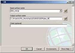
The edited DEM grid must be filled before producing a flow direction map.

From the Arc Toolbox, select Spatial Analyst Tools| Hydrology | Fill. Enter dem_merge for Input surface raster and adddem_fill to the end of the Output surface raster field.

24. 

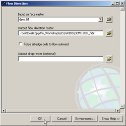
Produce a flow direction grid from the filled DEM grid.

From the Arc Toolbox, select Spatial Analyst Tools | Hydrology | Flow Direction. Select dem_fill as the Input surface rasterand enter 120m_fldir as the Output flow direction raster. Click OK.

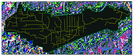
25. Create a watershed raster.

From the Arc Toolbox, select Spatial Analyst Tools | Hydrology | Watershed. Select 120m_fldir for Input flow direction raster. For the Input raster or feature pour point data field, click the Open  button and navigate to the outlet point shapefile located as follows: \GIS\outlet.shp. Select Id for Pour point field, and enter wshed as theOutput raster. The resulting display may resemble the image below:

26. 

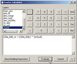
Create a flow direction grid constrained by the watershed raster.

Use the Raster Calculator to evaluate the following expression:

120m_fldir_w = [120m_fldir] * [wshed]

27. Export the flow direction grid as an ASCII file for import to Vflo™.

From the ArcToolbox, select Conversion Tools | From Raster | Raster to ASCII. Select 120m_fldir_w for Input raster and Output ASCII raster file to:\Vflo\ASCII\flow_direction.asc.

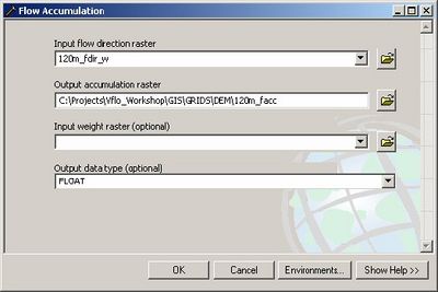
28. Produce a flow accumulation grid from the flow direction grid.

From the ArcToolbox, select Spatial Analyst Tools | Hydrology | Flow Accumulation. Select 120m_fldir_w for the Input flow direction raster and enter 120m_facc as the name of the Output accumulation raster. The Output data type may be FLOAT. Click OK.

29. 

Create a stream grid from the flow accumulation grid.

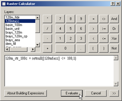
This stream grid will represent where channel cells will be located in Vflo™. To create the stream grid, the setnull Raster Calculator function will be used. This function evaluates an input grid, setting all values that evaluate to be true to “NoData,” and setting all other values to 1. “100”, or approximately 1.5 sq km, will be established as the “river threshold.”

Use the Raster Calculator to evaluate the following function:

120m_str_100c = setnull([120m_facc] <= 100, 1)

The stream grid 120m_str_100c is now ready to be exported from ArcGIS and imported into Vflo™ to identify channel cells, if desired.

 

30. 

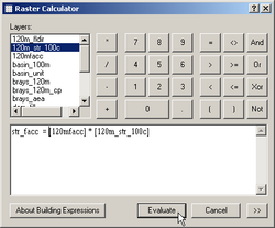
Produce a new stream grid whose values are represented by flow accumulation.

Use the Raster Calculator to multiply the stream grid by the flow accumulation grid, as follows:

str_facc = [120m_facc] * [120m_str_100c]

Channel width

Before using this section, see Parameter map formatting requirements for general ASCII formatting instructions.

This section includes tutorial instructions for using GIS software to produce a channel width map for input to Vflo™. In a distributed model, channel characteristics must be specified. One approach is to derive a geomorphic relationship between drainage area and channel bottom width, as described in the tutorial instructions below. Channel width parameters may also be determined from as-built plans or surveys, or deduced from local knowledge about channels, as well.

Developing a channel width map using GIS effectively establishes the location of channel cells in the Vflo™ model. If more detailed channel characteristics are known (i.e. area-stage and stage-discharge rating curves, or cross section data), then they can be added at specific locations while retaining the trapezoidal definition of the basic channel cell elsewhere.

Tutorial instructions

1. Insert a new data frame.

Select Insert | Data Frame. Scroll within the Table of Contents to the New Data Frame and rename the data frame Channels.

2. Set the projection to Albers Equal Area.

Double click on Channels and select the Coordinate System tab. Within the Select a coordinate system field, select Predefined | Projected Coordinate System | Continental | North America │ USA Contiguous Albers Equal Area Conic USGS version. Click OK.

3. Outside of ArcMap, open \GIS\Grids\ and make a new folder called Channels.

4. Update the working directory to \GIS\Grids\Channels.

From the Spatial Analyst toolbar, select Spatial Analyst │Options │General. Click the Open  button next to the Working Directory field and navigate to\GIS\GRIDS\Channels. Click OK.

5. Copy the layers str_unit and str_facc from the DEM Processing map and paste them in the Channels data frame.

Right click on str_unit within the Table of Contents and select Copy. Then right click on the Channel data frame and select Paste Layer. Repeat for str_facc.

6. Compute the drainage area for each channel cell.

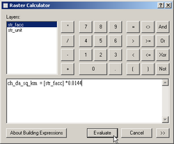
Using the Raster Calculator, multiply the drainage area of each cell (120m = 0.0144 km²) by the channel flow accumulation map, str_facc, as below. The following expression is only valid for a cell resolution of 120m.

ch_da_sq_km = [str_facc] * 0.0144

7. Generate the channel width grid.

Use the Raster Calculator to 

multiply the drainage area raster, ch_da_sq_km, by the relationship indicated below. This expression is only valid for this basin. Relationships for other basins must be based upon that basin’s characteristics. Name the resulting layer ch_width.

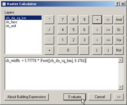
Metric units: ch_width = 5.77778 * Pow([ch_da_sq_km], 0.1782)

US Customary units ch_width = 5.77778 * Pow([ch_da_sq_km], 0.1782) / 0.3048

8. Export the channel width grid as an ASCII file for import to Vflo™.

From the ArcToolbox, select Conversion Tools | From Raster | Raster to ASCII tool. Select ch_width for Input raster, and Output ASCII raster file to\Vflo\ASCII\channel_width_meters.asc (or \Vflo\ASCII\channel_width_feet.asc, if US Customary units are used).

Channel side slope

Before using this section, see Parameter map formatting requirements for general ASCII formatting instructions.

Tutorial instructions

1. Create a channel side slope grid where all values are equal to 2.

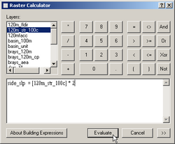
Use the Raster Calculator to multiply the stream grid by 2 in accordance with the equation below:

side_slp = [120m_str_100c] * 2

If geomorphic relationships between side slope and drainage area are available, a distributed map of side slope can be computed based on the flow accumulation.

If you are going through these instructions sequentially, you may need to activate the DEM Processing data frame in order to access the 120m_str_100c layer. Right click on DEM Processing and select Activate, then complete Step 1 as described above.

2. Export the channel side slope grid as an ASCII file for import to Vflo™.

Within the ArcToolbox, select Conversion Tools | From Raster | Raster to ASCII tool. Output ASCII raster file to \Vflo\ASCII\channel_side_slope_2_1.asc.

Slope

Before using this section, see Parameter map formatting requirements for general ASCII formatting instructions.

Tutorial instructions

1. Insert a new data frame (Insert│Data Frame) and label the data frame Slope.

2. Set the projection as desired.

3. Copy the layers listed below from the DEM Processing data frame to the Slope data frame.

Right click on each layer and select Copy. Right click on the Slope data frame and select Paste Layer.

a. High resolution DEM (brays_aea)

b. Stream flow accumulation (str_facc)

c. Stream polyline shapefile (brays_channels_aea)

4. Set resolution to a high resolution DEM.

Select Spatial Analyst│Options │ Cell Size. Select Same as Layer “brays_aea” for Analysis cell size.

5. Create a slope grid from the high resolution DEM.

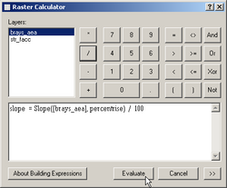
Use Raster Calculator to calculate the following expression:

slope = Slope([brays_aea], percentrise) / 100

Note that this grid represents overland slope as a decimal fraction. Slope maps for Vflo™ must be expressed as a non-percentage (decimal fraction), not in degrees from horizontal.

6. Resample the overland slope grid to the Vflo™ model resolution.

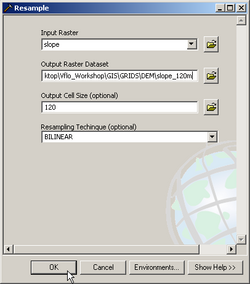
Within ArcToolbox, select Data Management Tools | Raster | Resample tool. Select slope for Input Raster. Navigate to\GIS\GRIDS\DEM\slope_120m for Output Raster Dataset. Enter 120 for Output Cell Size. Select BILINEAR for Resampling Technique.

7. Set the extent and cell size to the desired output Vflo™ domain.

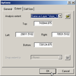
Select Spatial Analyst│Options│Extent. Choose Same as layer “slope_120m” from the Analysis extent drop down menu.

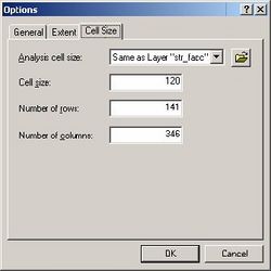
Within the same Options window, click on the Cell Size tab and select Same as layer “str_facc” from the Analysis cell sizedrop down menu.

8. Clip the resampled slope layer to the Vflo™ domain.

Use the Raster Calculator to evaluate the following expression:

slope_cp = [slope_120m]

9. Export the slope grid as an ASCII file for import to Vflo™.

Within the ArcToolbox, select Conversion Tools | From Raster | Raster to ASCII tool. Select slope_cp for Input raster and Output ASCII raster file to\Vflo\ASCII\slope_dec.asc.

Roughness

Before using this section, see Parameter map formatting requirements for general ASCII formatting instructions.

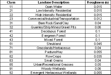
An integer-based classification system is used for landuse data sets, where each integer in the grid represents a landuse class (e.g. forest, urban, grassland, etc.) These landuse classes must be joined with actual roughness values using Spatial Analyst. For example, an area described as commercial on a landuse map is classified as Class 23, then joined with a roughness value of 0.012 using Spatial Analyst.

Tutorial instructions

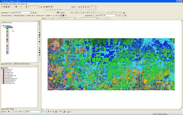
1. Insert a new data frame (Insert│Data Frame) and label the data frame Roughness.

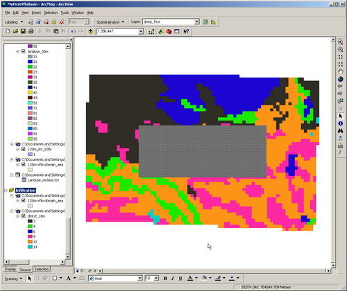
2. Load the files listed below into the Roughness data frame using the Add Data  button:

a. Landuse parameter map: \GIS\GRIDS\Roughness\landuse_30m

b. Vflo™ domain: \GIS\120m-vflo-domain_aea.shp

c. Stream threshold raster: \GIS\GRIDS\DEM\str_100

The resulting display may resemble the image below:

 

3. Load the landuse reclassification table by clicking the Add Data  button and navigating to GIS\Tables\Landuse_reclass.txt.

The reclassification table below shows the information included in the Landuse_reclass text file. It represents the conversion between the National Land Cover Data (NLCD/Anderson) landuse description and Manning’s roughness values.

 

4. Join the landuse raster to the roughness table.

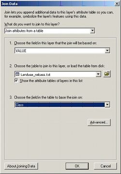
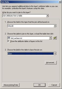
Right click on the landuse layer, landuse_30m, and select Joins and Relates | Join. In the Join Data dialog box, select the following:

Join Attributes from a table

Field 1: VALUE

Field 2: Landuse_reclass.txt

Field 3: Class

5. 

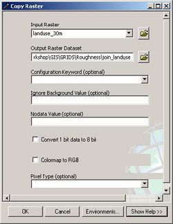
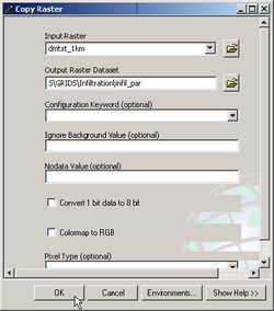
Add the roughness values permanently to the landuse parameter map.

Within the ArcToolbox, select Data Management Tools | Raster | Copy Raster. Set the Input Raster to landuse_30 and change the name of the Output Raster Dataset to join_landuse. Ignore the remaining optional fields and click the OK button.

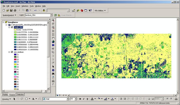
6. Create the roughness raster.

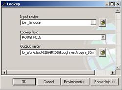
Within the ArcToolbox, select Spatial Analyst Tools | Reclass | Lookup. Set Input Raster to join_landuse. Set Lookup fieldto ROUGHNESS. Enter Output raster as rough_30m.

The resulting display may resemble the image below.

 

7. Resample the 30m roughness grid to 120m.

Within the ArcToolbox, select Data Management Tools | Raster | Resample. In the Resample window:

a. Select rough_30m as the Input Raster

b. Name the Output Raster Dataset rough_120m

c. Set Output Cell Size to 120

d. Choose BILINEAR for Resampling Technique

8. Set the extent and cell size to that of the landuse grid.

Select Spatial Analyst | Options | Extent and choose Same as Layer “120m-vflo-domain_aea.shp” for Analysis extent.

Then, remaining within the Options window, click on the Cell Size tab. Select As Specified Below for Analysis cell size and set Cell size to 120.

Finally, click on the General tab and make sure that the Working directory field still shows \GIS\GRIDS\Roughness.

9. Clip the re-sampled roughness raster to the Vflo™ domain.

Select Spatial Analyst │Raster Calculator. Multiply rough_120m by “1”. Name the new layer rough_120m_cp.

10. Create a uniform channel roughness map.

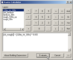
Use Raster Calculator to multiply the channel raster map, 120m_str_100c, by a uniform value of “0.015”. Name the new layerch_rough.

11. Merge the channel roughness raster with the overland roughness raster.

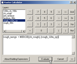
Enter the following equation in the Raster Calculator:

rough_merge= MERGE([ch_rough], [rough_120m_cp])

12. Export the merged roughness grid as an ASCII file for import to Vflo™.

Within the ArcToolbox, select Conversion Tools | From Raster | Raster to ASCII tool. Select rough_merge for Input raster and Output ASCII raster file to\Vflo\ASCII\merged_roughness.asc.

Infiltration

Before using this section, see Parameter map formatting requirements for general ASCII formatting instructions.

This section includes instructions for developing hydraulic conductivity, wetting front, and effective porosity parameter maps. These three infiltration parameters are used in Vflo™ to calculate infiltration using the Green-Ampt equation.

Soil texture datasets use an integer-based classification system, in which each integer in the grid represents a soil type class (e.g., clay loam, loamy clay, silty clay loam, etc.). These soil type classes must be joined to infiltration parameters such as effective porosity, saturated hydraulic conductivity, and wetting front suction head values usingSpatial Analyst. For example, sandy loam soil is assigned a class of 3, which must then be joined to an effective porosity value of 0.412 using Spatial Analyst.

For these instructions, the State Soil Geographic Database, STATSGO, was used to obtain infiltration parameters. STATSGO is a geographic database archived by the USDA Natural Resources Conservation Service (NRCS) containing soil data for the entire United States. The dominant soil texture grid was used to obtain Green-Ampt infiltration parameters such as saturated hydraulic conductivity, effective porosity and wetting front suction head. Other soil datasets are available for specific locations, including the NRCS Soil Survey Geographic Database, SSURGO; the NRCS MIAD/MUIR dataset; the United Nations Food and Agriculture Organization (FAO) soil maps; and others.

Tutorial instructions

1. Insert a new data frame (Insert | Data Frame). Click twice on the data frame to rename it: Infiltration.

2. Load the files listed below into the Infiltration data frame using the Add Data  button:

a. Soil Texture parameter map: \GIS\GRIDS\Infiltration\dmtxt_1km

b. Vflo™ domain: \GIS\120m-vflo-domain_aea.shp

The resulting display may resemble the image below:

 

3. Load the infiltration reclassification table.

Click the Add Data  button. If you are using US Customary units, navigate to GIS\Tables\Soil_reclass_US.txt. If you are using metric units, navigate toGIS\Tables\Soil_reclass_Metric.txt.

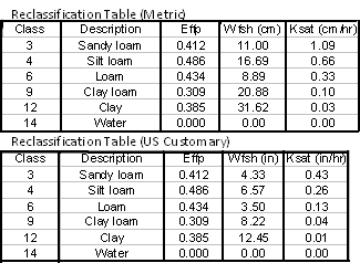
The reclassification table below shows the Green and Ampt infiltration parameters of the Unified Soil Classification System that are included in the Soil_reclass text files.Effp stands for Effective Porosity, Wfsh stands for Wetting Front Suction Head, and Ksat stands for Hydraulic Conductivity.

Note that these values are for illustrative purposes and should be replaced with values representative of the particular watershed being modeled.

4. Join the soil map to the infiltration table.

Right click on the soil layer, dmtxt_1km, and select Joins and Relates | Join. In the Join Data dialog box, make the following selections:

Join attributes from a table

Field 1: VALUE

Field 2: Soil_reclass_US.txt or Soil_reclass_Metric.txt

Field 3: Class

5. To add the infiltration values permanently to the soil map, copy the soil raster.

Within the ArcToolbox, select Data Management Tools | Raster | Copy Raster. Set the Input raster to dmtxt_1km and change the name of the Output Raster Dataset to infil_par. Ignore the remaining optional fields and click the OK button.

 

6. Create the hydraulic conductivity raster.

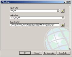
Within the ArcToolbox, select Spatial Analyst Tools | Reclass | Lookup. Set Input Raster to infil_par. Set Lookup field toKSAT_CM_HR if metric units are used, or KSAT_IN_HR if US Customary units are used. Enter the Output raster asksat_cm_hr or ksat_in_hr.

7. Create the wetting front suction raster.

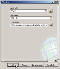
Within the ArcToolbox, select Spatial Analyst Tools | Reclass | Lookup. Set Input Raster to infil_par. Set Lookup field toWFSH_CM if metric units are used, or WFSH_IN if US Customary units are used. Enter the Output raster as wfsh_cm orwfsh_in.

8. Create the effective porosity raster.

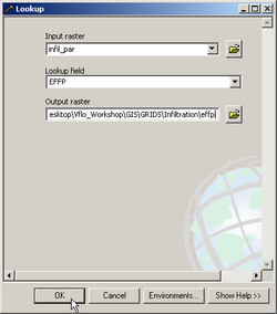
Within the ArcToolbox, select Spatial Analyst Tools | Reclass | Lookup. Set Input Raster to infil_par. Set Lookup field toEFFP. Enter the Output raster as effp.

9. Set the extent and cell size to match that of the Vflo™ domain.

Select Spatial Analyst | Options | Extent and choose Same as Layer “120m-vflo-domain_aea.shp” for Analysis extent.

Then, remaining within the Options window, click on the Cell Size tab. Select As Specified Below for Analysis cell size and set Cell size to 120.

Finally, click on the General tab and make sure that the Working directory field still shows \GIS\GRIDS\Infiltration.

10. Clip the resampled parameter rasters to the Vflo™ domain.

Select Spatial Analyst│Raster Calculator. For the hydraulic conductivity raster, multiply ksat_cm_hr (or ksat_in_hr) by "1", naming the new layer ksat_cm_hr_cp (orksat_in_hr_cp).

Repeat for the wetting front suction raster, wfsh_cm (or wfsh_in), and the effective porosity raster, effp.

11. Export the infiltration parameter maps as ASCII files for import to Vflo™.

Within the ArcToolbox, select Conversion Tools | From Raster | Raster to ASCII. For the hydraulic conductivity raster, select ksat_cm_hr_cp (or ksat_in_hr_cp) for Input raster and Output ASCII raster file to \Vflo\ASCII\ksat_cm_hr.asc (or ksat_in_hr.asc.)

Repeat for the wetting front suction raster, with Output to \Vflo\ASCII\wetting_front_suction_cm.asc (or wetting_front_suction_in.asc.)

Repeat for the effective porosity raster, with Output to \Vflo\ASCII\effective_porosity.asc.

Impervious

Before using this section, see Parameter map formatting requirements for general ASCII formatting instructions.

Tutorial instructions

1. Insert a new data frame (Insert│Data Frame) and name the data frame Impervious.

2. Impervious datasets may be in a raster or shapefile format, or they may be in ASCII format.

If the impervious dataset is in a raster or shapefile format, use the Add Data  button, navigate to the grid or shapefile, and click Add. For these instructions, navigate to the impervious shapefile \GIS\brayslulc_aea.

If the impervious dataset is in ASCII format, use the ArcToolbox to convert the ASCII to a raster format. Within ArcToolbox, select Conversion Tools | To Raster | ASCII to Raster. Select the impervious ASCII file for Input ASCII raster file, insert the desired name for the Output raster, and select FLOAT for Output data type.

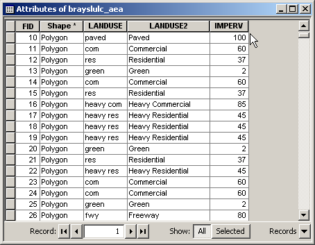
3. Convert the impervious shapefile, brayslulc_aea, to a raster grid populated by impervious percentage values.

There are seven landuse classes included in the brayslulc_aea file, as may be seen by viewing the brayslulc_aea attribute table (right click on brayslulc_aea, selectOpen Attribute Table.) Classes include: green, residential, heavy residential, commercial, heavy commercial, paved, and freeway. These classes have been assigned impervious percentage values, as seen in the attribute table column IMPERV.

 

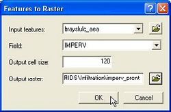
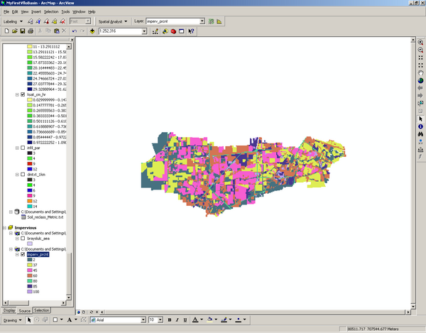
To convert the shapefile to a grid, select Spatial Analyst | Convert | Features to Raster. Select brayslulc_aea as Input features. Choose IMPERV for Field. Enter 120 for Output cell size. Name the Output raster imperv_prcnt.

The resulting display may resemble the image below:

 

4. Convert the impervious percentage values in imperv_prcnt to decimals.

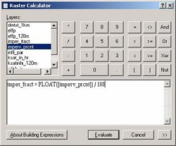
Vflo™ requires percentage-based parameter maps such as slope, impervious, and initial saturation to be in decimal format when they are imported as ASCII files.

Use the Raster Calculator to divide the impervious grid by "100". Use the Float function because the grid contains integer values:

imper_fract=(FLOAT([imperv_prcnt]) / 100)

5. Export the impervious grid as an ASCII file for import to Vflo™.

Within the ArcToolbox, select Conversion Tools | From Raster | Raster to ASCII. Select imper_fract for Input raster and Output ASCII raster files to\Vflo\ASCII\impervious_dec.asc.