Tutorial 3: Model calibration

There are many methods for calibrating a basin and improving simulated hydrographs. This tutorial describes one possible, general approach. Users are encouraged to research additional methods, and to consult the references listed here. For a full description of calibration in Vflo™, see the Calibration page.

This tutorial expands on the calibration skills developed in the tutorial Calibrating estimated parameters, guiding the user through the process of calibrating a real basin. For simplicity, hydraulic conductivity is not considered in this calibration exercise, as the model basin is highly urbanized. Hydraulic conductivity is set to a small, constant value. The roughness parameter, however, will need to be calibrated in order to match the simulated Vflo™ hydrograph to the observed hydrograph.

Preparing Vflo™ to run simulations

1. Load the basin model.

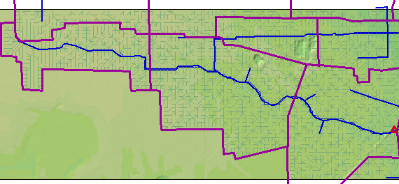
Select File | Open (or use the shortcut key CTRL+O, or the Open tool) to open an existing BOP or BOPX file. Navigate to the directory where the Vflo™ tutorial files are kept, and select \Tutorial3\Tutorial-3-Basin.bop. Make sure that BOP Files is selected for the Files of type field. Click Open. The basin model will be shown in the Main Display, as below.

2. Load precipitation.

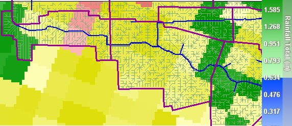
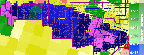
Select Precipitation | Load Precipitation | Existing RRP File | Browse and navigate to the file \Tutorial3\Tutorial-3-Rainfall.rrp. (Alternatively, use the Load precipitation tool.) Rainfall totals for the rainfall event loaded will be mapped in the Main Display, as shown below.

To view the rainfall hyetograph for any cell, select the cell using the Selection tool, then open the Precipitation panel.

Zooming to watch points

1. Click on the Watch Points list, located within the Cell List pane on the lower left of the Vflo™ interface.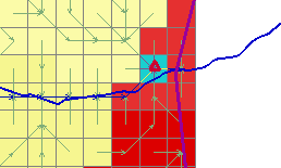

A single watch point, Roark Rd., has been established. To zoom to the watch point, click on the name Roark Rd., then select the Zoom button located at the top of the Watch Points list. The watch point cell, marked by a red triangle (default setting), will be selected.

Loading observed data for watch points

1. Ensure that the Roark Rd. cell is selected, as described above.

2. Select Tools | Load Observed Data for cell and navigate to the file \Tutorial3\Tutorial-3-Observed-english.txt. Click OK.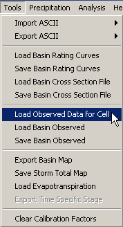

Loading observed data allows for observed data to be plotted on the simulated hydrographs, facilitating comparison of observed and simulated results for calibration. For further information, see Using observed data.

Note: the file Tutorial-3-Observed-metric.txt is included for the convenience of users employing metric units.

Checking calibration factors

Before solving Vflo™, it is important to observe what, if any, calibration factors are being applied to model parameters. This is especially important as the Hydraulics and Infiltration panels reflect base, rather than calibrated, values, as explained by the section Clearing calibration factors.

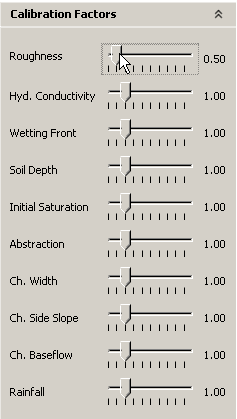
1. Open the Calibration Factors panel.

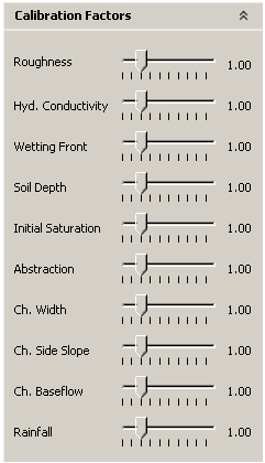
Verify that all calibration factors are set to "1.00". Using the Selection tool, select a few different cells at random to ensure that calibration factors are the same for all cells.

Checking the basin Network Analysis and cell properties

Conducting Network Analysis at the basin outlet prior to calibration may be useful, as it reports the range and mean of upstream cell parameters. To check the parameters of individual cells, the Hydraulics and Infiltration panels are used.

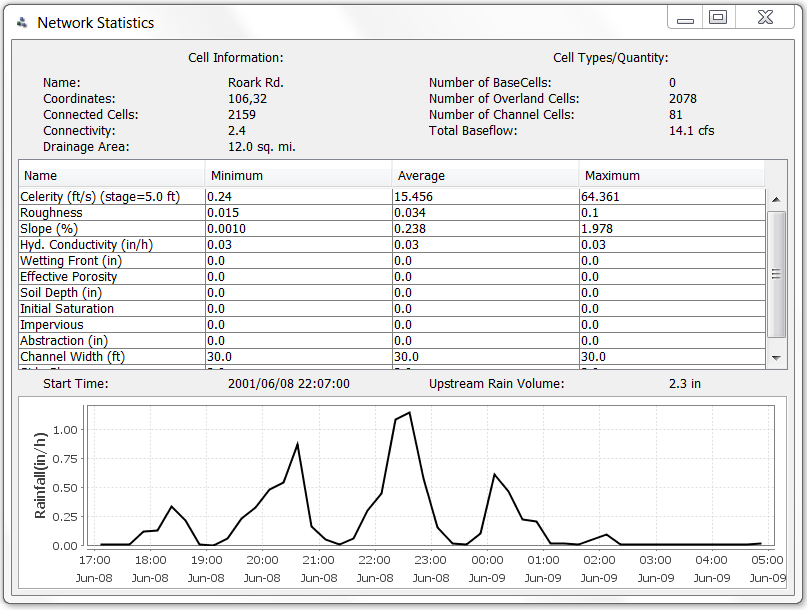
1. Select the Roark Rd. cell and press F1 to view the basin Network Statistics.

(Alternative methods: select Analysis | Network Analysis, or select the Network Analysis tool from the Vflo™ Toolbar.)

Notice that the baseflow is already set at 14 cfs (0.4 cms), and is distributed along the entire channel from cell (32,11) to the Roark Rd. watch point. If interested in observing the effect of baseflow on a Vflo™ simulation, the following instructions on calibrating roughness may be completed for the baseflow parameter.

2. To check individual cells, open the Hydraulics panel.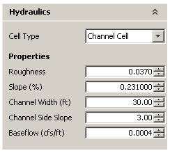

Click on the Hydraulics panel, then select a few cells at random to observe the cells' parameter values.

For the purposes of this exercise, note differences between the roughness values of overland cells and the roughness values of channel cells. If you suspect that either overland or channel cells are too rough or smooth, make a note of your observations, as they will be useful for the calibration process.

Calibrating roughness

 1. Solve Vflo™ at the watch point.

Using the Selection tool, select the Roark Rd. watch point (or, within the Watch Points list, click the Roark Rd. name, then click the Zoom button).

Press F5 (or select Analysis | Analyze Cell). In the Analysis Options window, enter a prediction length of 24 hours, then click Finish.

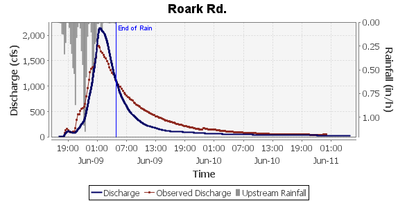
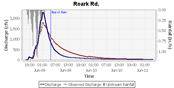
A stage hydrograph and a discharge hydrograph will be generated. Discard the stage hydrograph by clicking on the X in the upper right corner of the window. Your discharge hydrograph should resemble the figure below.

2. Evaluate differences between simulated and observed hydrographs.

Vflo™ plots the simulated hydrograph in black, and the observed hydrograph in red. Notice the differences between the two hydrographs. The time to peak is simulated a few hours late; the simulated falling limb is too steep; and the simulated peak discharge is too low. Based on these observations, adjustments to roughness will help improve the agreement between simulated and observed hydrographs.

If desired, take screen shots of each hydrograph generated in the calibration process. This may facilitate intercomparisons of hydrographs produced with different calibration factors.

3. Try decreasing roughness uniformly across the basin.

Click the Selection tool, then click the Select upstream cells tool. Finally, click the Roark Rd.cell to select all cells upstream of the watch point.

Alternatively, use the shortcut key CTRL, while clicking on the Roark Rd. cell.

Open the Calibration Factors panel. Click and drag the Roughness slider tab to the left, to a calibration factor of "0.5". (Note: Use the left and right arrows on your keyboard to adjust calibration values by 0.01 increments.)

Solve Vflo™ as described above. Compare the discharge hydrographs. Compared to the first hydrograph generated, the simulated hydrograph has been shifted to the left (i.e., lowering roughness made the peak arrive earlier); this has put the simulated and observed peaks in phase. The simulated hydrograph produced has steep rising and falling limbs, however, and a peak discharge that is much larger than the observed peak.

Overall, these observations indicate that decreasing roughness uniformly across the basin will not result in a good hydrograph match. Other parameter adjustments will need to be made.

4. Try decreasing roughness for channel cells only.

Adjust all cells upstream of Roark Rd. back to a roughness calibration factor of "1.0". With all upstream cells selected, adjust the Roughness slider tab back to "1.0".

Now, decrease the roughness values of the channel cells, only. To select only upstream channel cells (excluding all other cell types), choose the Selection tool and the Select upstream channel cells tool. Then, click on the Roark Rd.cell.

Alternatively, hold the shortcut keys CTRL+ALT while clicking the Roark Rd. cell.

In the Calibration Factors panel, adjust the Roughness slider tab to "0.5".

Solve Vflo™ and compare the discharge hydrographs. Notice that the simulated hydrograph is shifted left, without much increase in peak discharge.

To determine the next possible calibration steps, ask:

Is the peak discharge coming early enough?

Are the rising limbs a good match?

5. Continue adjusting channel roughness, with the goal of matching simulated and observed hydrographs.

Increase and/or decrease the channel roughness calibration factor as desired, until satisfied with channel roughness. Using increments no smaller than 0.05 is recommended until narrowing in on a final value. With each adjustment, solve Vflo™ and compare hydrographs.

6. Once satisfied with channel roughness, try increasing roughness for overland cells.

To select only upstream overland cells, click both the Selection and the Select upstream overland cells tools from the Vflo™ Toolbar before clicking the Roark Rd. cell.

Increase the Roughness calibration using the Calibration Factors panel, as desired.

Solve Vflo™ and compare the discharge hydrographs. Increasing overland roughness has the effect of lowering the peak discharge and flattening out the rising and falling limbs.

7. Continue to adjust channel and overland roughness separately, until satisfied with hydrograph results.

Calibration results and discussion

Although the process of calibration can be subjective, the roughness calibration factors that produce the "best" simulated hydrograph are:

Overland roughness: 1.50

Channel roughness: 0.50

The hydrograph obtained with these calibration factors is shown below.

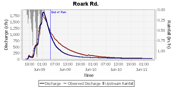
Prior to calibration, upstream roughness values were 0.034. In this watershed, the main channels are lined with concrete, and have a lower Manning's roughness coefficient than overland cells. Applying a roughness calibration factor of 0.35 to channel cells made channel roughness coefficients used in the routing calculations approximately 0.019, which is consistent with a concrete or asphalt channel. Applying a roughness calibration factor of 1.50 to overland cells made overland roughness coefficients approximately .051, which is consistent with vegetated land use.

These roughness values are appropriate for the basin being modeled: Brays Bayou, TX. The environment of Brays Bayou, located in Houston, TX, is that of an urban stream. Most of the channel has been modified with concrete lining and trapezoidal cross-sections (for which the channel widths and side slopes are well known, and incorporated into the model). Thus, the calibrated roughness values applied are consistent with the urban environment of the modeled basin.