Tutorial: Calibrating estimated parameters

Calibration is an important step in building a Vflo™ model, especially if parameter values have been estimated. This tutorial introduces the Calibration Factors panel in Vflo™, and demonstrates how simulated hydrographs are affected by changes in roughness and infiltration.

Peak discharge, volume, and timing are affected differently by parameter variations. The two parameters that may have the largest impact on these hydrograph properties are roughness (commonly symbolized by the letter n; also referred to as Manning's roughness) and hydraulic conductivity (commonly symbolized by the letter k). Altering these parameters to better match an observed hydrograph is the basis for model calibration.

For detailed information on calibration in Vflo™, see the Overview: Calibration page. For instructions on using the Calibration Factors panel, see the section on Using the Calibration Factors panel.

Preparing Vflo™ to run simulations

1. Run Vflo™ and select File | Open to open an existing BOP file.

Alternatively, use the Open tool, or the shortcut key CTRL + O.

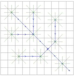
Navigate to the directory where the file is contained, and select Tutorial_2_basin.bop. Click OK. Your basin should resemble the figure at right.

Blue arrows represent channel cells, and green arrows represent overland cells (unless changes have been made to the Cell Colors settings, as described in Changing cell colors).

2. Observe the basin parameter values.

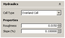
Choose the Selection tool from the Vflo™ Toolbar and click on a cell with a green arrow (an overland cell).

Then, click on the Hydraulics panel. Hydraulic properties are set to default values when the model is first opened. Overland cells have a default roughness of 0.015 and a slope of 0.1%. A Manning's roughness coefficient of 0.015 corresponds to a concrete or paved surface.

Now, using the Selection 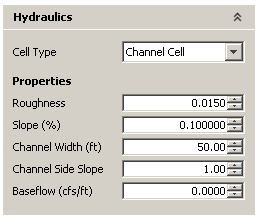tool, click on a cell with a blue arrow (a channel cell). Verify that, like the overland cell, the channel cell has a roughness of 0.015 and a slope of 0.1%. In addition, the channel cell has a channel width of 50 ft (15.24 m) and a 1:1 side slope.

3. Load the rainfall file tutorial-2-rain.rrp.

Select Precipitation | Load Precipitation, or click the Load precipitation tool. Choose the Existing RRP File option, click Browse, and navigate to the location of tutorial-2-rain.rrp. Click Next to return to the subbasin.

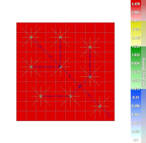
The rainfall file loads uniform rainfall over the 10x10 basin, for a total of 2.5 inches per cell over six hours.

4. Solve the drainage network at the outlet cell.

Using the Selection tool, select the outlet cell, located at (9,9) in the grid.

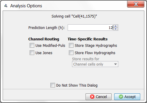
Then, select Analysis | Analyze Cell (or use the shortcut key F5, or the Analyze cell tool). Enter a prediction length of 12 hours in the Analysis Options window. Since this is a small, idealized basin, the rainfall will not take long to travel downstream.

5. Save the hydrograph results.

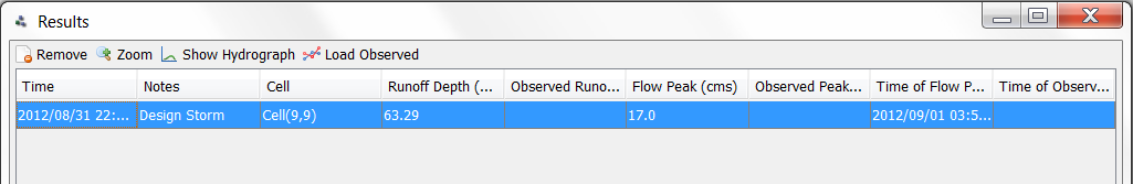
After saving, the Results window will appear, as shown below. To view the stage and discharge hydrographs for the solve, double click on the solve row, or select the solve row and click the Show Hydrograph button, as shown below.

Close the stage hydrograph window. In the discharge hydrograph window, select File | Save Textual Output. Save the text file in an appropriate location, and give it a distinct name such as discharge-no-calibration.txt.

Calibrating roughness

1. Select all cells in the basin.

With both the Selection tool and the Select upstream cells tool selected, click on the outlet cell (9,9).

2. Then, open the Calibration Factors panel.

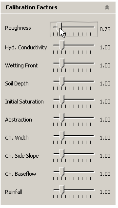
All calibration factors will be set to 1.00.

Click and drag the roughness slider tab to the left until the calibration factor reads "0.75". Use the left and right (and up and down) arrow keys on your keyboard to adjust the calibration factor by 0.01. Decreasing the roughness calibration factor to 0.75 means that the next time Vflo™ solves, the Manning's roughness value used in the routing calculations will be 75% of the base value, or

3. Solve Vflo™ at the outlet cell, as described above, and save the discharge hydrograph results.

Repeat steps 1 through 3 with the roughness calibration factor set at 1.5 and at 3.0.

4. Plot all four hydrographs in Excel or a similar data analysis software program, as shown below.

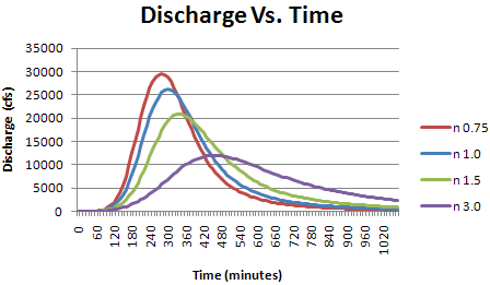
Roughness calibration discussion

A lower roughness calibration results in a larger peak discharge and a quicker time to peak. However, the volume of water being routed remains the same. As an exercise, you may consider integrating the area under the hydrographs to convince yourself that volume is nearly constant.

Also, it is worth investigating separately calibrating channel and overland cells. Adjusting the channel roughness changes the time to peak with minor attenuation. Calibrating overland roughness alters the shape of the hydrograph dramatically, causing both peak and timing to be affected. The exact effect depends on the basin properties.

When calibrating roughness, keep in mind the base values in your watershed. You should try to avoid a low calibration factor that produces an unrealistic Manning's roughness coefficient (i.e., below 0.01).

Calibrating hydraulic conductivity

1. Select all cells in the basin.

With both the Selection tool and the Select upstream cells tool selected, click on the outlet cell (9,9).

2. To enter a hydraulic conductivity parameter, open the Infiltration panel.

Click the Infiltration panel, then click within the Hyd. Conductivity field. Enter a value of 0.43 in/hr (10.9 mm/hr) for hydraulic conductivity.

3. Adjust the roughness calibration factor back to 1.00.

Open the Calibration Factors panel. Click and drag the roughness slider tab to the right, to the original value of 1.00.

4. Adjust the hydraulic conductivity calibration factor.

Click and drag the hydraulic conductivity slider to the left, to a value of 0.01. This will reduce the hydraulic conductivity by two orders of magnitude, so that the model represents impervious soil, or concrete.

5. Generate hydrographs with different hydraulic conductivity calibration factors.

Solve Vflo™ at the outlet cell, as described above, and save the discharge hydrograph results.

Solve Vflo™ and save the results three more times, with hydraulic conductivity calibration factors of 0.3, 1.0, and 5.0. These calibration factors result in simulation of runoff over loam, sandy loam, and sand, respectively.

6. Plot the hydrographs in Excel or a similar data analysis software program.

Hydraulic conductivity calibration discussion

Adjusting hydraulic conductivity affects how much rainfall is infiltrated into the soil, and how much becomes runoff. Therefore it should make sense that for dense soils (such as clay) the runoff is greater than for soils with higher infiltration rates (such as sand). The graph above shows that as hydraulic conductivity increases, the volume of runoff decreases, as does the peak discharge. Time of peak, however, is virtually unchanged.

Note that in the case of sand (where the calibration factor is set to 5.0), the infiltration rate always exceeds the rainfall and there is no runoff.

Several other parameters affect infiltration, in addition to hydraulic conductivity. Soil depth, for example, is included in Vflo™ as an infiltration parameter for the purpose of simulating saturation excess. Once the porosity of the soil is filled, then all rainfall is assumed to runoff. The initial saturation parameter affects how quickly the capacity of the soil to infiltrate will be exceeded. For a full description of all infiltration parameters, see the Infiltration parameters page.