Tutorial: Developing a Vflo™ model without GIS

This Tutorial demonstrates how to establish a Vflo™ domain, draw in flow direction arrows, and change cell types to build a basin model directly within Vflo™. The basin model will be saved as a BOP, or basin overland properties, file (*.bopx, *.bop). Other options for building a Vflo™ model include developing a Vflo™ model using AutoBOP and/or using GIS software to develop parameter maps for import to Vflo™.

The Tutorial also demonstrates the basic process of loading rainfall and generating hydrographs in Vflo™. Rainfall event data will be loaded as an RRP, or rainfall rate properties file, and hydrographs will be generated to demonstrate how the relative percentage of channel versus overland flow cells affects the hydrograph shape and response magnitude. Increased channelization accelerates the flow of runoff from cell to cell, causing higher peak discharge and earlier time to peak. This effect may or may not represent actual conditions.

This exercise may be used to demonstrate the effects of urbanization where natural surfaces are converted to urban land uses with concrete and asphalt surfaces and channelized flow. Agricultural drainage accomplished by building channels into poorly drained areas for purposes of conveying surface and subsurface runoff to an outlet may also be demonstrated using this exercise.

Establishing a Vflo™ domain

1. Run Vflo™ and select File | New (or press CTRL+N) to create a new basin.

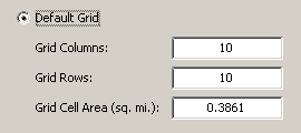
Within the Domain Wizard window, select the Default Grid option. Create a 10 column by 10 row basin, giving each cell an area of 1 square kilometer (or, approximately 0.386 square miles).

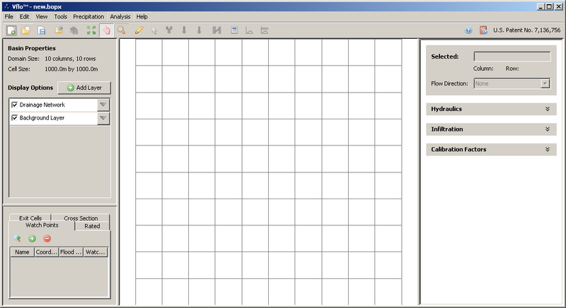
Click Next. You should now have a screen that looks like the example below.

Drawing in flow direction arrows

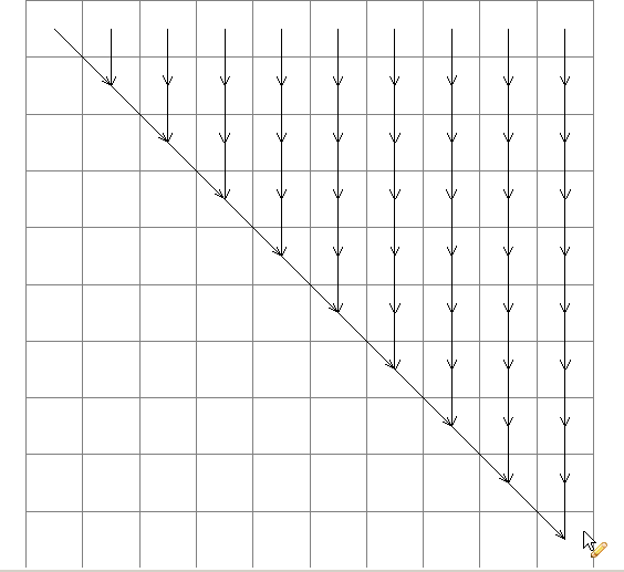
1. Manually connect the grid cells to create a drainage network as seen in the figure below.

To draw a flow direction arrow, select the Draw cell connections tool located in the Vflo™ Toolbar.

Click on a cell and drag the mouse to a neighboring cell. A black arrow will appear, originating from the first cell and pointing toward the second, neighboring cell.

Continue this process until the flow direction map is completed.

Changing cell type

1. Change all cells from default base cells to channel cells.

To select all cells, first click the Selection tool located in the Vflo™ Toolbar. Then, select the Select upstream cells tool. Both tools will be highlighted, as shown below.

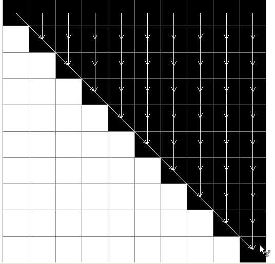
Finally, click on the outlet cell (9,9). All upstream cells will be highlighted.

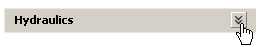
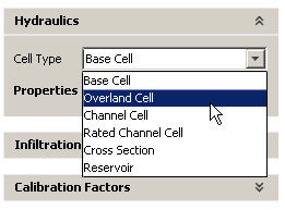
Then, click the Hydraulics panel, located in the Cell Properties pane on the right-side of the interface.

Find the Cell Type field, and change the selection from Base Cell to Overland Cell. All cells will become overland cells.

Saving the Vflo™ model as a BOP file

1. Once a basin model is developed, it is important to save the information in BOP format.

To save the basin model, select the Save tool located in the Vflo™ Toolbar.

Within the Save BOPX File window, select the desired directory and file name, then click Save.

Loading rainfall files

1. Load the rainfall file tutorial-1-rain.rrp.

Click the Load precipitation tool located in the Vflo™ Toolbar. In the Rainfall Wizard dialog, choose Existing RRP File.

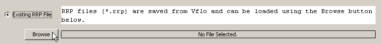
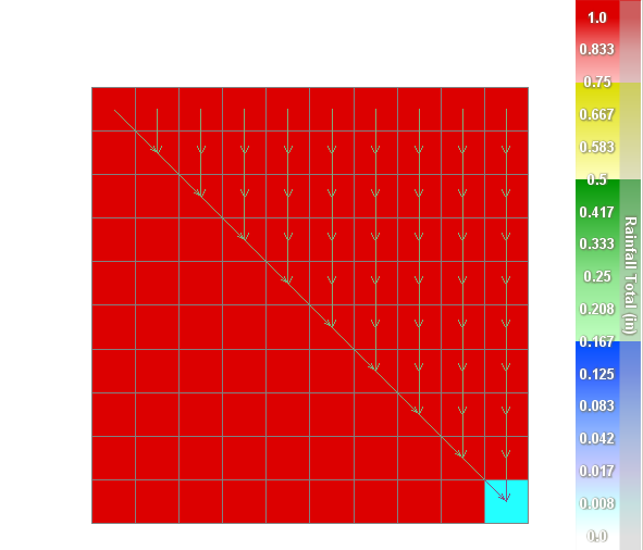
Within the Load RRP File window, browse to the file tutorial-1-rain.rrp, and click Open. After rainfall files are loaded, a rainfall total map is overlaid on the model grid in the Main Display, as shown below. (To replace the rainfall total map with other parameter maps or background images, see the instructions on Choosing the background layer of the Main Display.)

2. View a cell hyetograph.

To observe the hyetograph for any cell in the grid, select the desired cell and open the Precipitation panel, located within the Cell Properties paneon the right-side of the interface.

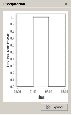
Note: the Precipitation panel is only visible after precipitation files have been loaded into Vflo™.

Solving Vflo™ to generate hydrographs

1. Solve Vflo™ at the outlet cell.

Select the outlet cell (9,9), then click the Analyze Cell tool located in the Vflo™ Toolbar.

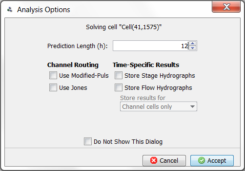
Within the Analysis Options window, enter a prediction length of 12 hours. Since this is a small, idealized basin, the rainfall will not take long to travel downstream. Leave all other options unchecked, and click Finish.

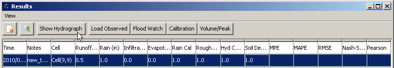
2. Vflo™ will generate a statistical Results report.

For a full explanation of the Results report, see Interpreting Vflo™ results.

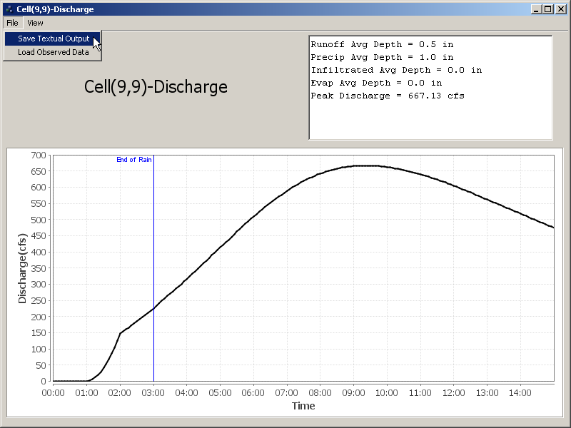
To view the stage and discharge hydrographs for the cell, click on the solve row so that it is highlighted, as shown below. Then, click the Show Hydrograph button.

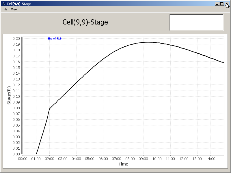
Two new windows will appear: a stage hydrograph and a discharge hydrograph. You may discard the stage hydrograph by clicking the X in the upper right corner.

The discharge hydrograph will look like the figure below. To save the hydrograph data as a text file, click File | Save Textual Output. Save the text file in an appropriate location, giving it a distinct name such as All Overland.txt.

Observing channelization effects

1. Demonstrate how increasing channelization affects simulated hydrographs.

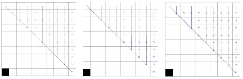
Re-solve Vflo™ three more times, increasing the number of channel cells (channelization) with each simulation.

Use the images below as a rough example of which cells to change.

Save the textual output with a descriptive name after each simulation (e.g., Main Channel.txt, 50% Channel.txt, All Channel.txt).

2. Compare the hydrographs.

Import the saved text files into Excel or a similar data analysis/graphing program, and evaluate the differences in the hydrographs by plotting all four hydrographs in a single graph, as shown below.

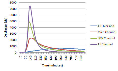
The combined hydrograph demonstrates that as more channel cells are added, the simulated hydrograph changes shape dramatically. The rising limbs are steeper and the peak is earlier and higher.

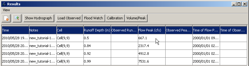
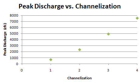
3. Determine the peak discharge value for each hydrograph.

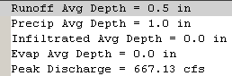
Peak discharge (Flow Peak) values are exported along with other key statistical information and can be found at the top of the hydrograph text file, as shown at right. In addition, peak discharge values may be found in the Volume/Peak report, as shown below.

Plot peak discharge against degree of channelization, as shown by the graph below. It is apparent that peak discharge increases with increasing amounts of channelization.

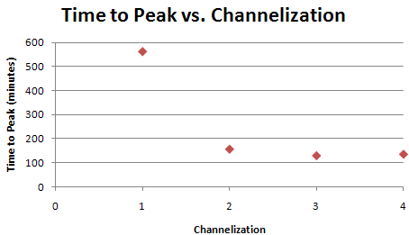
4. Determine time to peak for each hydrograph.

Time to peak (Time of Flow Peak) information may be obtained from the Volume/Peak report, as shown above. Plot time to peak against degree of channelization, as shown by the graph below. As demonstrated, time to peak decreases with increasing amounts of channelization.

Tutorial summary

This exercise demonstrates how important cell classification is in determining accuracy of runoff routing based on hydrodynamics. Under- or over-representation of channel cells in Vflo™ will have a large impact on simulation accuracy. The user should exercise care that a sufficiently detailed channel network is well represented. Every channel in the watershed does not need be modeled as a channel. However, the proportion of channel to overland flow cells affects the simulated results. As a general rule, around 10% of the watershed should be represented as channel cells.