Model Theoretical Background
The digital watershed shown below is composed of finite elements that connect grid cells according to principal drainage direction. The connectivity of the finite elements forms the basis for solving the kinematic wave, or conservation equations. The conservation equations are used to model explicitly the hydraulic components of the drainage network.
Overland flow, channel hydraulics, storage-discharge relationships for detention basins, complex channel cross-section, stage-discharge rating curves, and shallow water wave propagation are combined where appropriate to model the digital watershed. This hydraulic approach to hydrology closely couples runoff generation and losses with the routing of this runoff through the drainage network. As such it is a departure from traditional methods, such as the unit hydrograph, where runoff generation and routing are artificially separated. This page presents the mathematical analogy and numerical algorithms that provide the foundation for physics-based distributed (PBD) hydrologic modeling using conservation of mass and momentum.

Hydrologic and environmental processes are distributed in space and time. Simulation of these processes is made possible through the spatial data analysis and management techniques of GIS. Vflo™ uses digital maps of soils, land use, topography, and rainfall to compute rainfall runoff generation and routing in each grid cell in the drainage network.
Runoff generation is caused by rainfall rates exceeding infiltration rates, called soil profile saturation. Runoff losses due to infiltration in channels are typical to alluvial fans in more arid climates, or to karstic geology in areas where fractures permit runoff arriving from upstream to percolate into the subsurface.
Analytic solutions to the equations governing runoff are not generally obtainable, giving rise to the need for numerical methods such as finite element or finite difference methods 1. Jayawardena and White (1977, 1979), Ross et al. (1979), and Kuchment et al. (1983, 1986), among others, use the finite element method to solve the governing equations on equivalent cascades, planes, or sub-areas with homogeneous properties 2 3 4 5 6. The solution using linear, one-dimensional elements presented by Vieux et al. (1988, 1990) uses a single chain of finite elements for solving overland flow 7 8. This solution differs from previous finite element solutions because it represents roughness and slope as nodal rather than elemental parameters. This difference in approach enables the simulation of spatially variable watershed surfaces without the need to break the watershed into equivalent conceptual cascades, planes, or sub-areas.
The PBD model called r.water.fea is a finite element approach to watershed modeling that explicitly represents spatially variable input and parameters. The model was developed in 1993 for the U.S. Army Corps of Engineers, Construction Engineering Research Laboratory, Champaign, Illinois (CERL). The goal was to provide a hydrologic modeling tool that used GIS maps of parameters directly within the GIS environment. Initial development of the model is part of the public domain GIS called GRASS (Geographic Resource Analysis Support System).
Vieux and Gauer (1994) extend the r.water.fea finite element solution to a network of elements representing a watershed domain with channels within a GIS environment 9. Later modifications include channel routing, a Green and Ampt infiltration routine, and distributed radar rainfall input.
In Vflo™, finite elements are laid out in the direction of the principal land-surface slope, consistent with the kinematic flow analogy. Unlike most finite element applications where high element density is used to resolve large gradients or complex geometry, the elements used by Vflo™ are one-dimensional elements with lengths consistent with the grid-cell resolution. This constant resolution supports the parameterization of the nodal finite element parameters using GIS maps with grid-cell values. Through linkage of the raster data structure and the nodal finite element method, the grid-cell value becomes the nodal value in the finite element solution.
The goal of distributed hydrologic prediction is to accurately represent the spatial and temporal characteristics of a watershed that govern the transformation of rainfall into runoff. Thus, distributed hydrologic modeling relies on geospatial data used to define topography, landuse/cover, soils, and precipitation input. Distributed hydrologic modeling may be termed physics-based if it uses conservation of momentum, mass, and energy to model the processes. Most physics-based distributed (PBD) models solve a flow analogy (e.g. kinematic, diffusive wave, or full dynamic) with numerical methods using a discrete representation of the catchment, such as a finite difference grid or finite element mesh. Besides r.water.fea, described in Vieux and Gauer (1994) and Vieux (2004), other PBD models include: the Vflo™ distributed hydrologic model (Vieux and Vieux, 2002; Vieux et al., 2003); CASC2D (Julien and Saghafian, 1991; Ogden and Julien, 1994); Systeme Hydrologique Européen (SHE) (Abbott et al., 1986 a;b); and the Distributed Hydrology Soil Vegetation Model (DHSVM) (Wigmosta et al., 1994)9 10 11 12 13 14 15 16 17.
Of these PBD models, r.water.fea and Vflo™ employ the finite element method. Both the r.water.fea and the Vflo™ models rely on geospatial data and GIS analysis to generate parameter maps, but while r.water.fea requires the Geographic Resource Analysis Support System (GRASS) and runs as a GIS function, Vflo™ does not require a GIS to run the model. This does not mean that integration within a GIS is not possible: Vflo™ features specifically facilitate integration within ArcGIS, supporting analysis of geospatial data, extraction of the drainage network, and creation of distributed parameter maps. With the exception of drainage direction, nodal parameters of the finite element solution used in Vflo™ are taken from the GIS raster of gridded values to develop integrated basin models.
A DEM is used to configure the drainage network; flow direction for each finite element and nodal slope values are derived from the DEM. Consequently, the connectivity of the drainage network is used to develop the system of equations that provide a solution to the kinematic wave analogy. Besides being an efficient means for solving the kinematic wave equations, the finite element method provides an intuitive approach in which arrows (1-D finite elements) are laid out between grid cells in the direction of principal slope. The figure below shows a 3x3-cell patch in order to demonstrate the grid-cell scheme used to define the finite elements connecting overland flow and channel elements.

The delineated network is referred to as D8, meaning that there may be up to eight flow directions that converge on a single cell, as shown in the figure below. Flat or divergent flow areas where the flow direction is indeterminate must be resolved through GIS analysis procedures before such cells may be incorporated into the solution. The resolution of the DEM determines the fundamental length scale for routing water over the land surface and through channels.

Mathematical formulation
The kinematic wave analogy (KWA) for overland flow is a simplification of the conservation of mass and momentum equations wherein the principle gradient is the land surface slope. Lighthill and Whitham (1950), as well as many others, have explored the application of these simplified equations to describe flood waves in rivers18. The mathematical analogies are simplifications of the full form of the momentum conservation equation. The velocity, V, and the flow depth, y, in a prismatic channel are associated by these relationships:
Equation 1:
Kinematic: 
Diffusion: 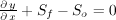
Dynamic: 
in which Sf and So are the friction and bedslope gradients, respectively. The kinematic wave analogy depends on the bottom slope and friction gradient. More terms are included in the diffusion analogy and dynamic forms of the equation. If all other terms are small, or an order-of-magnitude less than the bed slope or friction gradient, the KWA is an appropriate representation of the wave movement downstream (Chow et al., 1988)19. The simplified momentum equation and the continuity equation may be written for both channel and overland flow. The one-dimensional continuity equation for overland flow resulting from rainfall excess is expressed by:
Equation 2: 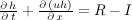
in which R is rainfall rate; I is infiltration rate; h is flow depth; and u is overland flow velocity. In the KWA, we equate the bed slope with the friction gradient. In open channel hydraulics, this amounts to the uniform flow assumption. Using this fact together with an appropriate relation between velocity, u, and flow depth, h, such as the Manning equation, we obtain,
Equation 3: 
in which So is the bed slope or principal land surface slope, and n is the hydraulic roughness. Velocity and flow depth depend on the land surface slope and the friction induced by the hydraulic roughness. For this reason, the KWA analogy enforces that:
- The slope of the water surface and friction gradient are parallel with the land surface slope
- Flow is uniform, and
- Backwater is not permitted.
Substituting Eq. 2 into Eq. 1 results in the KWA equation for relating flow depth to the land surface slope, hydraulic roughness, rainfall and infiltration rates:
Equation 4: 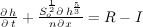
When written in terms of h, Eq. 4 is applicable to overland flow. The slope and hydraulic roughness are spatially variable, while rainfall, infiltration and flow depth are both spatially and temporally variable. For channelized flow, Eq. 2 can be written with the cross-sectional area A instead of the flow depth h, as in:
Equation 5: 
in which Q is the discharge or flow rate in the channel, and q is the rate of lateral inflow per unit length in the channel. Channel cross-sectional characteristics and the Manning equation are used to solve Eq. 5 analogously to Eq. 4. The KWA is appropriate to most conditions encountered in a watershed. Eqs. 4 and 5 are the governing equations for overland and channel flow, respectively. If backwater or flat slopes are prevalent, the diffusive wave analogy (DWA) is more appropriate to the solution. The following sections demonstrate numerical solutions to Eqs. 4 and 5 for a grid-cell representation of the watershed.
Finite element solution
The finite element method is an efficient way to transform partial differential equations in space and time into ordinary differential equations in time. Finite difference schemes may then be used to solve for the time-dependent solution of the system. Many different finite element solutions have been developed in the general field of engineering mechanics. Specifically, Galerkin’s formulation has been used to solve Eqs. 4 and 5 using 1-D linear elements (Vieux et al., 1988; Vieux et al., 1990; Vieux and Segerlind, 1989; Vieux and Gauer, 1994) 7 8 9 20.
Time-dependent solution
To solve Eq. 4 or 5 in time, a discretization scheme is needed, such as the finite difference scheme. The scheme should produce accurate and stable solutions. A continuous form is discretized by the finite difference formulation as follows:
Equation 6:
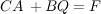
![$ CA_{new} = CA_{old} - \Delta\,t\,B[(1-\theta)Q_{old} + \theta\,Q_{new}] + \Delta\,t[(1-\theta)F_{old} + \theta\,F_{new}] $](/vflo-guide/sites/default/files/tex/8778189419262d2b1605b06c7e54e7dc450b05e5.png)
in which  is the weighting coefficient,
  is the time step, and the new and old subscripts denote the value of the variable at the next time step and current time step, respectively. The explicit solution
  has been chosen because it is faster than implicit schemes, even with the limiting time step of the Courant condition. The time step is a function of the Courant condition, which requires that the time step be less than the time of travel for a gravity wave to propagate across the element at celerity equal to
  at the deepest flow rate. The time step associated with the Courant condition is given as:
Equation 7: 
in which L is the length of the shortest element. The most restrictive element can be identified as that which has the shortest Courant time step. In practice, this is difficult to identify because the spatially variable rainfall and hydraulic characteristics of any given event may force different elements to be the most restrictive.
Rainfall excess determination
A right-hand forcing vector utilizes the rainfall excess at every time step. Rainfall excess at each grid cell is determined by rainfall rate minus infiltration rate. During a storm event and afterward for a specified monitoring period, the Green and Ampt equation computes the amount of infiltration. Comparison of rainfall rate to the potential infiltration rate determines whether all the rain infiltrates, or whether excess is available for routing to the next downstream cell. Any excess arriving from upstream at a particular cell location is added to the rainfall for that cell. In this way, runoff from upstream may infiltrate or add to the rainfall excess in each cell.
Equations 8 and 9, shown below, define runoff generated by infiltration rate excess. As long as the rainfall rate, i, is less than the potential infiltration, the cumulative infiltration is simply equal to rainfall rate integrated over the time period, as shown in:
Equation 8: 
As soon as rainfall exceeds the potential infiltration, water starts ponding at the surface. From this point, the cumulative infiltration is defined as,
Equation 9: 

Saturation excess is modeled when the soil porosity is filled, i.e., the wetting front reaches the soil depth. After each day, the infiltrated volume is redistributed in the soil profile and the degree of saturation recomputed. Potential rate of evapotranspiration depletes soil moisture.
Soil moisture computations
During continuous simulations in order to accurately determine cumulative runoff volume, soil moisture is continuously tracked in each cell. Soil moisture is determined from the infiltrated volume that is redistributed at the end of each day from the wetting front volume. This soil moisture is depleted at the potential rate of evapotranspiration and the crop coefficient map if applied. In continuous simulation, soil moisture is replenished by subsequent infiltration from rainfall and depleted at the potential rate subject to the crop coefficient map. The timeseries of soil moisture at each watch point is reported in the Continuous Simulator output that is the average of upstream cells.
Distributed maps of flow and infiltration
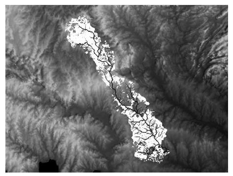
An option exists in the solve dialog (F5) for saving distributed maps of stage, discharge or infiltration depth. If checked, these options will increase the solve time because of extensive read/write of output maps. Only use this option to save when the model is running satisfactorally and distributed output is needed. An example of a distributed runoff map produced at 270 meter resolution for the 1200 km2 Blue River basin is shown below. The map shown is for a particular time interval of one hour during an event simulated using radar rainfall input. The flow depth is draped on a 3-D rendering of the digital terrain model. Darker areas represent deeper flow depths, while lighter areas represent shallower flow depths. The drainage network is apparent in this image because of the accumulation of runoff downstream of the more intense rainfall. There are areas where there is no runoff, caused by low rainfall rates during this particular time period and/or soils that have infiltration rates that exceed the rainfall rate.
Summary
Physics-based distributed modeling achieves a close coupling of runoff generation and the routing of this runoff through a drainage network. This approach is achieved through a hydraulic approach to hydrology, which is a departure from traditional methods where runoff generation and routing are artificially separated. The mathematical analogy and numerical algorithms described are the foundation for modeling runoff at any location in a watershed.
Flow direction and slope derived from a DEM are used to solve the kinematic wave equations. The direction of principal slope classified according to the eight neighboring cells defines the connectivity used to assemble a system of equations. Using the finite element method to solve the kinematic wave analogy and GIS maps of parameters with rainfall input, the runoff process is simulated.
- 1. Singh, V.P. and D.A. Woolhiser, 2002. Mathematical modeling of watershed hydrology, J. Hydrol. Eng. 7(4): 270-292.
- 2. Jayawardena, A.W. and J.K. White, 1977. A finite element distributed catchment model (1): Analysis basis, J. Hydrol. 34: 269-286.
- 3. Jayawardena, A.W. and J.K. White, 1979. A finite element distributed catchment model (2): Application to real catchment, J. Hydrol., 42: 231-249.
- 4. Ross, B.B., D.N. Contractor, V.O. Shanholtz, 1979. A finite element model of overland and channel flow for accessing the hydrologic impact of land use change, J. Hydrol. 41: 11-30.
- 5. Kuchment, L.S., V.N. Demidov and Yu.G. Motovilov, 1983. Formirovanie rechnogo stoka: fisikomatematicheskie modeli (River runoff formation: physically based models) (in Russian), Nauka, Moscow.
- 6. Kuchment, L.S., V.N. Demidov and Y.G. Motovilov, 1986. A physically based model of the formation of snowmelt and rainfall runoff. In: Modelling Snowmelt-Induced Processes (Proc. Budapest Symp., July 1986), IAHS Publ., 155:27-36.
- 7. a. b. Vieux, B.E., V.F. Bralts, L.J. Segerlind, 1988. Finite element analysis of hydrologic response areas using geographic information systems, Am. Soc. Civ. Eng.
- 8. a. b. Vieux, B.E., V.F. Bralts, L.J. Segerlind, and R.B. Wallace, 1990. Finite element watershed modeling: One-dimensional elements, J. Water Resour. Plann. Manage. 116(6): 803-819.
- 9. a. b. c. Vieux, B.E. and N. Gauer, 1994, Finite-element modeling of storm water runoff using GRASS GIS. Microcomputers in Civil Engineering 9: 263-270.
- 10. Vieux. B.E. 2004. Distributed Hydrologic Modeling Using GIS, Second Edition, Springer, Water Science Technology Series, 48, ISBN 1402024592.
- 11. Vieux, B.E. and J.E. Vieux, 2002. Vflo™: A Real-time Distributed Hydrologic Model. Proceedings of the 2nd Federal Interagency Hydrologic Modeling Conference, July 28-August 1, 2002, Las Vegas, Nevada. Abstract and paper on CD-ROM.
- 12. Vieux, B.E., C. Chen, J.E. Vieux, and K.W. Howard, 2003. Operational deployment of a physics-based distributed rainfall-runoff model for flood forecasting in Taiwan. HS03: International Symposium on Information from Weather Radar and Distributed Hydrological Modeling, IAHS General Assembly at Sapporo, Japan, July 3-11, 2003. Submitted paper, IAHS, Red Book Series.
- 13. Julien, P.Y. and B. Saghafian, 1991. CASC2D user manual – a two dimensional watershed rainfall-runoff model. Civil Engineering Rep. CER90-91PYJ-BS-12, Colorado State University, Fort Collins: 66.
- 14. Ogden, F.L, and P.Y. Julien, 1994. Runoff model sensitivity to radar rainfall resolution. J. Hydrol.', 158: 1-18.
- 15. Abbott, M.B., J.C. Bathurst, J.A. Cunge, P.E O’Connell, and J. Rasmussen, 1986a. An introduction to European Hydrological System –Systeme Hydrologique Europeen, “SHE”, 1 History and philosophy of a physically-based distributed modeling system., J. Hydrol., 87, 45-59.
- 16. Abbott, M. B., Bathurst, J. C., Cunge, J. A., O’Connell, P. E., Rassmussen, J., 1986b. An Introduction to the European Hydrological System- Systeme Hydrologique European, “SHE”, 2: Structure of a Physically-Based Distributed Modelling System, J. Hydrol., 87: 61-77.
- 17. Wigmosta, M. S., L. W. Vail and D. P. Lettenmaier, 1994. A Distributed Hydrology-Vegetation Model for Complex Terrain. Water Resour. Res., 30(6): 1665-1679.
- 18. Lighthill, F. R. S. and Whitham, G. B., 1950. On Kinematic Waves, I, Flood Measurements in Long Rivers. Proceedings of the Royal Society of London, (229), pp.281-316.
- 19. Chow, V. T., Maidment, D. R., and Mays, L. W., 1988, Applied Hydrology. McGraw-Hill, New York.
- 20. Vieux, B.E. and Segerlind, L.J., 1989, “Finite element solution accuracy of an infiltrating channel”. In: Finite element analysis in fluids, Proceedings of the Seventh International Conference on Finite Element Methods in Flow Problems, April 3-7, 1989, Edited by: Chung, T. J., and Karr, G.R., The University of Alabama in Huntsville, Alabama,:1337-1342.